The PF Interval is a key concept when selecting preventive maintenance tasks. But with more and more equipment being fitted with real-time asset health monitoring equipment and with the advent of Predictive Analytics and Big Data, is it really relevant anymore? In this article, we will discuss the PF Interval, how it is applied and whether it can be applied to equipment fitted with real-time health monitoring and where equipment health is assessed using Predictive Analytics and Big Data.
What is the PF Interval?
Before starting, let’s give a brief introduction to the PF Interval.
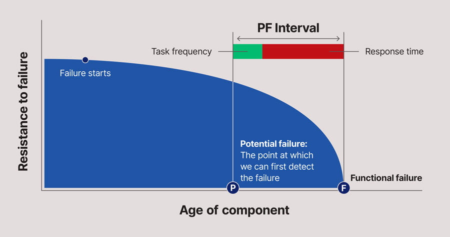
The term P-F interval is a core concept of Reliability Centered Maintenance (RCM) and was first coined by the late John Moubray in his book RCM II. In essence it was intended to illustrate a fairly simple concept associated with selecting a Condition-Based inspection (or Predictive Maintenance) task to deal with a specific failure mode, which was nonetheless not well understood at the time. It can be visualised as shown in the diagram below.
- The PF Curve applies at a Failure Mode level – that is, it applies to one Failure Cause. Some condition monitoring techniques (e.g. vibration analysis) may be able to detect mutiple failure modes, but each of these failure modes will have their own PF Curve.
- The point at which the failure starts need not necessarily be coincident with the item entering service. Indeed the incipient failure may be initiated by a random event, such as impact loading, a random overload etc.
- However, once the failure starts, then it is assumed that resistance to failure will continue to decrease over time.
- It may only be some time after the point at which the incipient failure has been initiated that we can first detect that the failure is occurring. This is called the point P on the curve – the point at which we can first detect the “Potential Failure” – a term which has a specific meaning in RCM terminology. Note that, at the point P, the equipment is still functioning – it has not yet suffered a “Functional Failure” (another RCM term with a specific meaning).
- Some time after the point P, the item will suffer a Functional Failure – it will no longer be able to fulfil its intended function. This is the point F on the curve.
- The time interval between the points P and F on the curve is called the “PF Interval”.
- To be effective, a Condition-Based inspection must be performed at a frequency that is less than the PF Interval (and sufficiently shorter than the PF Interval to give time to avoid the consequences of the Functional Failure).
- There are a few other requirements and/or assumptions that must be met before a Condition Based Maintenance task is appropriate. These include requirements for:
- The length of the PF Interval to be long enough to permit avoidance of the consequences of failure
- The length of the PF Interval must be “reasonably consistent” for the failure mode being considered.
Enhancements to the PF Interval concept
Since its initial development, others have enhanced and embellished this chart in various ways:
- Some have added additional points to the left of the “point at which the failure starts” in an attempt to indicate how design, installation and operation decisions can impact on equipment reliability. While potentially useful, my personal belief is that this muddies the picture, and detracts from the very simple message which the chart is intended to communicate.
- Some have attempted to quantify the relationship between “Resistance to Failure” and “Age” using statistical analysis. Besides the practical difficulties associated with obtaining enough data to be able to quantify this relationship (and the definitional issues concerning how to determine “resistance to failure”), obtaining an accurate representation of the PF Curve is, in almost all cases, of little practical value in assisting in avoiding the consequences of in-service failures. A “near enough” estimate of the PF Interval, allowing for some variation in its likely length, based on practical experience and judgement is all that is required in all but a few exceptional cases.
The PF Interval in the world of the Industrial Internet of Things (IIoT)
The PF Interval, as we have explained, assists with determining the frequency at which a periodic Condition-Based Inspection should be conducted. But what about the situation where, via the Industrial Internet of Things, equipment health is being continuously monitored, in real-time? How, if at all, does the concept of the PF Interval assist?
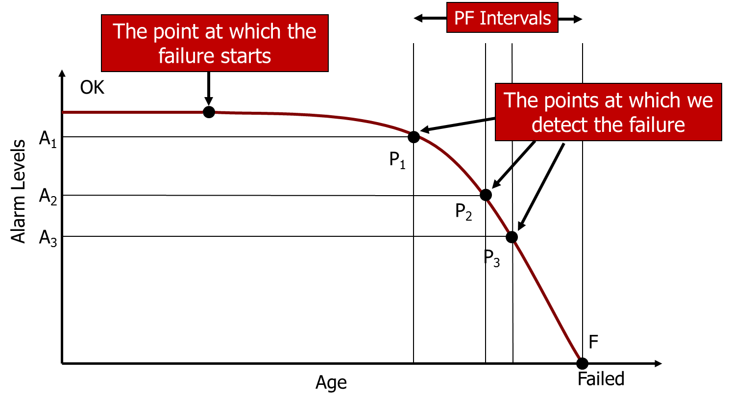
The short answer is that it is still useful – but in this case, not to determine the frequency of inspection, but to determine the level of “health” at which an alarm should be raised and action initiated. With continuous monitoring, we can choose the level at which an alarm can be raised. Clearly, the alarm needs to be raised sufficiently far before the point at which the item suffers a Functional Failure in order for us to be able to avoid or minimise the consequences of that Functional Failure. As illustrated below, different alarm levels will be associated with different points “P” on the PF Curve, and therefore different PF Intervals. Alarm Level A1 (associated with the Point P1) gives us the longest PF Interval, A2 gives us the next longest etc. What we should do is to first determine how much warning we need of an impending Functional Failure to be able to avoid or minimise its consequences, and then set the alarm level at a point that will give us the required amount of warning. For example, for a rolling element bearing, we could set the Alarm level for vibration to a relatively low level and this would give us a longer PF Interval, and therefore more warning of impending failure. This would be appropriate if, for example, the machine was production critical and the bearing was difficult to access, requiring extended warning to plan and schedule the required maintenance.
This is all eminently sensible, so long as we have some understanding of the shape of the PF curve and can therefore predict the P-F Interval – how much warning we get – at each alarm level setting. While we may have some intuitive understanding of this relationship, in the case of more sophisticated technologies, we may need a higher degree of accuracy (and more quantitative data) than our intuitive knowledge can provide. In this situation, some research and/or tests may be required in order to determine this relationship. This, of course, requires us to run equipment to failure (or at least very close to failure) either in the field or in a laboratory, which may or may not be feasible depending on the nature of the equipment and the consequences of those failures. We are starting to see this sort of testing and experimentation with some of our clients, though it remains a rarity.
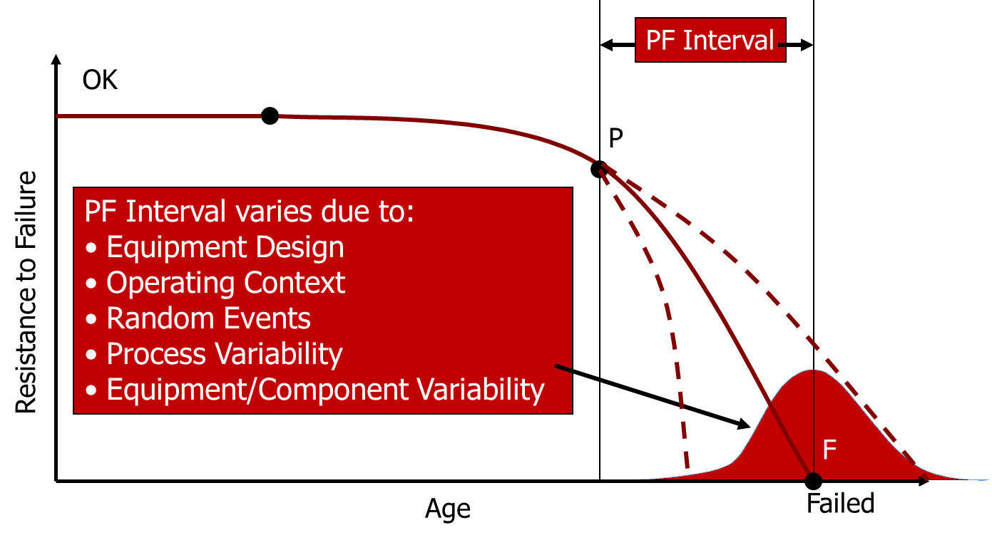
Obtaining a valid model of the PF curve becomes even more problematic when you consider that, for any given failure mode, it may vary depending on a number of factors, including:
- Equipment Design – was the equipment designed using a high or low factor of safety? How much margin is there in the design to cope with potential overloading?
- The Operating Context of the Equipment – how is the equipment being operated in comparison to the design intent? Is it subjected to factors such as periodic impact loading or high start/stop cycles that might affect the PF Interval?
- Random Events – what protections exist against random external events which could have an effect on component life (e.g. operator error, maintenance error, installation error etc.)?
- Process Variability – how often, and how large is the variation in load on the equipment?
- Equipment/Component Variability – the inevitable variability in the quality of manufacture of the equipment and its component parts, particularly where organisations are changing to cheaper sources of spare parts to “save money”.
These factors create variability in the PF Interval that can significantly affect the warning time provided by a particular alarm level, as indicated below:
This variability needs to be taken into account in any experiments or tests to determine the PF Interval and, as in-service failures are (hopefully) comparatively sparse, the research may take some considerable time to complete. In the meantime, we are still required to make an informed judgement about the appropriate Preventive Maintenance regime to implement.
The advantage, of course, is that in a world of real-time health monitoring, acquiring the data should be comparatively easy. We just need to make sure that we do collect it, and that we use it for this type of analysis. This requires genuine reliability engineering and data analysis skills that are relatively rare in most organisations.
The PF Interval in the world of predictive analytics and big data
One of the other key aspects of the PF Interval is that it relates to one failure mode at a time, and the output is one alarm level for one parameter of equipment health (e.g. vibration, or noise, or wall thickness etc.).
However, Big Data, as applied to failure prediction (for more on this topic see our article “Big Data, Predictive Analytics and Maintenance” uses data from more than one source to predict equipment failure. For example, a more sophisticated predictive analytics model may predict equipment failure for a truck engine if it sees a particular combination of oil degradation (from Oil Analysis), engine power loss (from the Engine Monitoring System and/or Refuelling bowsers) and text on Operator Pre-start sheets. In practice, how could we apply the PF Interval to either:
- Set the alarm limits for the Predictive Analytics model, or
- Know what the PF Interval will be for a particular alarm determined by the Predictive Analytics model?
The answer appears to me to be “not easily”, but it will depend on the type of Predictive Analytics model used. There are three fundamental families of models that can be used:
- Theoretical models. These are based on an understanding of the physics of failure, and measure and analyse the variables underpinning a theoretical model of failure in order to predict when that failure will occur. For example, for fatigue failures, we know that there is component life is determined by the level of applied cyclical stress and the number of cycles applied. If we measure those two parameters (applied cyclical stress and the number of cycles) for a given component, we should be able to predict when the component will fail.
- Regression models. These use various forms of statistical analysis, from simple linear regression models to multivariate adaptive regression models in order to predict that equipment failure is about to occur.
- Machine learning models. Put very simply, these emulate the way that humans learn by detecting patterns amongst variables that have, in the past, led to equipment failure, and then using pattern recognition techniques to identify situations similar to those that have occurred in the past.
For theoretical models, the concept of the PF Interval should be able to be comparatively easily applied. An alarm level should be able to be set based on the deterioration rate embedded in the model, and this should be able to be set so that it gives sufficient warning of impending failure to avoid or minimise the consequences of the Functional Failure.
For the other two models (Regression and Machine Learning), the relationship between alarm levels and the PF Interval will be much harder to determine. Indeed, with these types of models, there may be multiple types of alarms that all may have the same PF Interval. Unless the models can, in some way, be used to derive a prediction of the relationship between the parameters that make up the model and “Resistance to Failure” (i.e. plot the PF Curve), then it may be difficult to adjust the alarm level and understand what the impact of this adjustment on the PF Interval will be. To determine this relationship in multivariate models such as these may require an even greater amount of data (and an even greater number of failures) than would be required for simpler, single-variable models in order to arrive at conclusions that were statistically significant. In many applications, collecting and analysing this data may neither be practical nor justified.
However the general principle that the amount of warning we get must be long enough to allow us to avoid or minimise the consequences of the Functional Failure still holds – and all of these failure prediction models must abide by this requirement, otherwise they will provide no practical business benefits.
Conclusion
In summary, the PF Interval remains a vitally important conceptual model to assist people to understand one of the core concepts of RCM – how to determine the frequency of a simple Condition-Based Maintenance task. In terms of its application to predicting equipment failure using real-time equipment health monitoring sensors, it also has some conceptual application, but in practice may need further extension and development for more complex failure prediction situations. When considering the PF Interval in association with Predictive Analytics and Big Data for failure prediction, its use may be even more limited and/or complex. However the general principle embedded in the PF Interval concept – that the amount of warning we get of impending failure must be long enough to allow us to avoid or minimise the consequences of the Functional Failure – is entirely valid for all Predictive Maintenance tasks.
Your thoughts and comments are welcome. Please feel free to contact me to discuss this further.
Want further training in PF Interval and RCM principles?
As part of our Asset Management training suite, we offer a number of courses that deal with PF Interval and RCM concepts and principles. To view our course outlines, or register a spot for you or your team, see the course pages below.
-
Product on sale
 RCM & PMO for Team MembersOriginal price was: $2,150.00.$1,935.00Current price is: $1,935.00.
 -
Product on saleEffective Asset Management Strategies and PlansOriginal price was: $1,075.00.$967.50Current price is: $967.50.